Heirarchical Bayesian Analysis
Project Management
To run a heirarchical bayesian analysis, depending on the scale of the project we should start with the following output:
- EDA/Data QA meeting
- Goal
- review input data & confirm accuracy
- establish which hypotheses can be tested and the likely accuracy thereof
- determine the best/initial guess at the hierarchy structure
- Goal
- Analysis Results
- Goal
- Review relationships & performance goals
- Outline recommendations & potential upsides
- Identify how to improve within-channel effectiveness
- Goal
Data Preparation
We need two key inputs to get started:
- An existing model (or set of models) — this is usually our baseline aggregate-level model that we want to extend/enhance with hierarchy.
- Deep-dive media channel performance data — this dataset includes more detailed dimensions (e.g., campaign, ad product, placement, device,….). This deep-dive data can be the same dataset used before or a new, more granular one.
Main preparation tasks:
- Clean the data thoroughly (ensure we have only the data for the activity that is running: cross-check any new data Vs pervious more aggregate data).
- Explore the available data structures and possible hierarchies (e.g., campaign → ad product → placement → device).
- Use Chris’s data visualization scripts — these handy plots quickly show how the data is nested and help us visually pick the most sensible hierarchy to start with.
Choosing the right hierarchy early saves a lot of time and prevents modeling headaches later.
Model estimation
Once we have a clean dataset and a chosen hierarchy, we move to estimation:
- Append the hierarchical data to our existing model dataset so everything lives in one place.
- Use the econometrics tool we already have, which supports Bayesian analysis.
- Leverage Chris’s custom extension code — this is the key piece! The extension lets us:
- explicitly define the variable hierarchy we want to test
- automatically run a recursive loop of Bayesian model fits that move through the hierarchy levels
- produce clean, structured outputs ready for the HB Results Viewer
After the loop finishes, the results can be used to populate the HB results viewer tool (see below).
HB results viewer: Tool population
We have a specific hierarchical bayesian results viewer tool for working with HB models, which integrates the cost, activity, impact and clients specific financial return models with the results from a Heirachical Bayesian Model
The tool is available here: https://route1io.shinyapps.io/copilot_hierarchical_bayesian/
The purpose of the tool is to allow quick data QA and link the input data, heirarchical bayesian results, and financial return models into a single platform that allows us to calculate a series of bayesian-based financial return metrics for all the variables being considered.
The data for this tool is populated in a client-specific folder in the route1io.hierarchical.bayesian s3 bucket, and 3 input data files are required:
data.csv
This is the input data set for the variables being tested. The format of the file is very similar to the digital channel tool, but should be configured with the dimensions that are being investigated in the HB analysis. There are upto 4 levels of heirarchy supported within the analysis, and both input and response metrics can be added to the data set, even though not every fact will be used. Data should be input at the daily level.
The columns used in this data set should be:
- Date Column: a column containing the date for a given observation
- Hierarchy Definition Columns (upto 4): upto 4 heirarchical definition columns can be added into the analysis
- Metric Values: additional columns should be added to include Cost, Impressions, Clicks, Conversions (for example, platform tracked values) plus any additional metrics that may be useful for data exploration
response.csv
This is the file containing the results from a HB analysis for import into the tool. It is a combination of variables.csv from the econometric model analysis and the output from a HB analysis.
The columns used in this data set are:
- Hierarchy Definition Columns (upto 4): these should match the exact naming and values in the data.csv file and config.json file
- KPI: this is the kpi (model) that the response will be related to and should match the calculation inputs in the client’s financial return model
- HB values: these should be the coefficients and standard errors of the coefficients from the HB output. Note: these may need to be calculated to invert any mean-centering, pooling or other transformation on the dep vars in the model
- Data_mean, Data_se: the mean & se of the coefficient from the base model
- Prior_mean, Prior_se: the prior mean & se used in the analysis. For lower level hiearchical bayesian analysis, these are likely taken from the level-above
- Posterior_mean, Posterior_se: the posterior mean & se from the analysis.
- Variable Transformations: The transformation on the variable that is used in the model, taking the values from variables.csv in the econometric model tool
- Lag
- Decay
- Log
- RollingSum
- NegExp
- Asym
- xmid
- scale
- RF
- RP
- DR
The response.csv file needs to be structured so that we can see all direct or drill-down levels of results. To enable this, if the next levels down are not active for a given data entry, they should be left blank. This leaves you will a file that looks something like this:
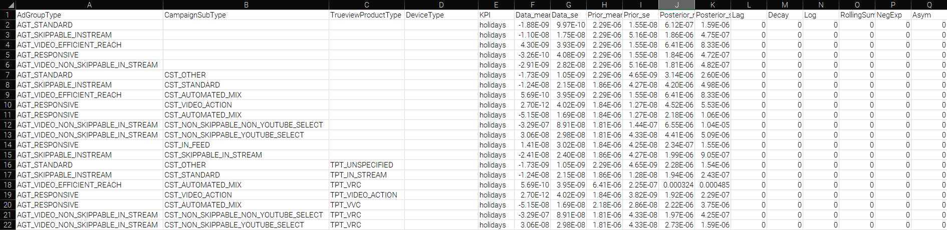
The column headers and options of the file should match the config.json file (see below). The KPI column in response.csv should have values that match the client-specific financial return model
config.json
this file contains the configuration settings for the tool and calculations, nested as follows
- Variable Names: these map the variable names used in the data.csv file to the underlying structure of the code base. They will also be used for display in the UI
- “date”: the field name of the date field
- Hierarchy Definition Columns: ordered from highest to lowest level of heirarchy
- “market”: top level
- “brand”: 2nd level
- “channel”: 3rd level
- “channel1”: 4th level
- Standard Variable definitions - additional fields are available but there should be a mapping for each of these metrics
- “clicks”
- “impressions”
- “cost”
- “conversions”
- Settings: these contain settings used in the app
- “default.currency.mark”: the string to use in front of a currency value
- “date.format”: the format that dates are saved in within a csv file (for example: “dmy”)
- “variable.units”: the untransformed units that the variable in the model is measured in (for example “impressions”. This needs to be available in data.csv
- “market.name”: the name of the market/country that this data represents. This is used to link to the correct financial return parameters
- Metrics: a list of metrics to be available for EDA
- Table Metrics: a list of metrics in the data set that should be included in EDA tables
An example of the config.r file format is shown below
{

  "variable.names": {

    "date": ["Date"],

    "market": ["AdGroupType"],

    "brand": ["CampaignSubType"],

    "channel": ["TrueviewProductType"],

    "channel1": ["DeviceType"],

    "clicks": ["Clicks"],

    "impressions": ["Impressions"],

    "cost": ["Cost"],

    "conversions": ["Conversions"]

  },

  "settings": {

    "default.currency.mark": ["£"],

    "date.format": ["dmy"],

    "variable.units":["Impressions"],

    "market.name":["UK"]

  },

  "metrics": [

    ["Impressions"],

    ["Clicks"],

    ["Cost"],

    ["CPM"],

    ["CPC"],

    ["CTR"],

    ["Conversions"],

    ["Cost per Conversion"]

  ],

  "table.metrics": [

    ["Cost"],

    ["Impressions"],

    ["CPM"],

    ["Clicks"],

    ["CPC"],

    ["Conversions"],

    ["Cost per Conversion"]

  ]

}
Methodology Approach: Using Hierarchical Bayesian Regression to Dissect Marketing Campaign Effectiveness
In modern marketing, campaigns often consist of multiple components—channels (e.g., TV, digital, social), creatives, messaging themes, offers, and targeting segments—running simultaneously across markets, time periods, or customer cohorts. A key analytical challenge is to separate the contribution of each component while properly accounting for varying sample sizes, correlations, and contextual differences.
Hierarchical Bayesian regression (also called multilevel or partial-pooling models) is one of the most powerful and flexible tools for this task. Instead of running dozens of separate A/B tests or fully pooled regressions (both of which can be misleading), hierarchical models let analysts start with high-level effects and progressively “drill down” into finer-grained components using informative, nested priors.
Core Idea: Shrinkage and Partial Pooling
Hierarchical models estimate parameters at multiple levels simultaneously:
- Level 1: High-level groupings (e.g., channels)
- Level 2: Components (e.g., specific partners)
- Level 3+: Sub-Components (e.g., ad placements, campaigns, or customer segments)
Lower-level parameters are regularized (shrunk) toward their group means, with the degree of shrinkage automatically determined by the data. Components with little data borrow strength from the broader population; high-volume components are allowed to deviate. This dramatically reduces false positives compared to classical null-hypothesis testing and gives more honest uncertainty estimates.
Modeling Campaign Components Hierarchically
A typical structure for dissecting a campaign might look like this in mathematical notation, followed by an R/brms or RStan implementation sketch:
Let
- yᵢ: outcome KPI (e.g., sales conversions)
- c[i]: channel (TV, Social, Search, etc.)
- p[i]: placement or publisher nested within channel
- r[i]: creative nested within publisher
To start, a baseline model of the outcome KPI as described by the channel-level (and other variable) effects would be established to understand overall channel performance.
From there, a hierarchical regression would be specified, using the level-above results as the prior to pass in to sequentially & recursively lower-level estimations
This recursive nesting structure is the key: creatives and publishers do not receive a single global prior; each is centered on its parent channel mean. The model can therefore answer:
- Does the Social channel as a whole underperform Search? (compare posterior estimates of impact and return between “Social” and “Search)
- Within Social, which partners or placements meaningfully outperform the channel average? (check whether 95% credible interval of β_placement[i] excludes zero)
Testing for Meaningful Differences
Use posterior probabilities and regions of practical equivalence (ROPE):
-
Pr(β_creative[j] > 0 data) > 0.95 → strong evidence of outperformance - 95% credible interval entirely within ±0.1 log-odds → practically equivalent to the group mean
Diagnostic Statistics and Remediation
In Bayesian regression using R (e.g., via rstanarm or brms), MCMC sampling approximates the posterior distribution. Convergence ensures samples from multiple chains mix well and represent the target posterior reliably. The Rhat (Gelman-Rubin) statistic quantifies this by comparing within-chain and between-chain variances:
- Relevance: Rhat ≈ 1 (ideally <1.05, max <1.1 across parameters) indicates chains have converged to the stationary posterior. Values >1.1 signal poor mixing—chains haven’t stabilized, leading to biased inferences (e.g., unreliable credible intervals for regression coefficients). It’s a chain-level diagnostic; compute via summary() or shinystan on fitted models like stan_glm().
Handling Rhat Issues
- If Rhat >1.1: Chains are “stuck” (e.g., multimodal posterior).
- Remediations (prioritize in order):
- Increase iterations: iter = 4000 (default 2000) or chains: chains = 4 (default 4). Rerun model.
- Thin samples: thin = 2 to reduce autocorrelation.
- Reparameterize: Center/scale predictors (scale = TRUE in stan_glm); use informative priors (e.g., prior = normal(0, 2.5) for coefficients).
- Switch samplers: Try NUTS with higher adapt_delta = 0.95 (default 0.8) to handle funnel geometries.
- Model simplification: Drop interactions or use hierarchical priors if overparameterized.
- Remediations (prioritize in order):
Other Key Diagnostics & Remediations
Monitor these post-fit via summary(fit), plot(fit), or launch_shinystan(fit). Aim for stable, efficient sampling.
| Diagnostic | What It Checks | Issue Threshold | Remediation Actions |
|---|---|---|---|
| Effective Sample Size (n_eff) | Independence of samples (accounts for autocorrelation). | <100 per chain (or <10% of total iter). | - Thin: thin = 5. - More warmup: warmup = 2000. - Reparameterize for lower autocorrelation (e.g., non-centered hierarchies). |
| Trace Plots | Visual chain mixing (should look like “fuzzy caterpillars,” not trends/wandering). | Trends, high variance between chains. | - Inspect: plot(fit, “trace”). - Increase chains/iter; check data for outliers (remove via robust priors like Student-t). |
| Autocorrelation Plots | Sample independence (lags should decay quickly). | Slow decay (>0.1 at lag 10). | - Thin samples. - Use stronger priors or simplify model (e.g., fewer predictors). |
| Divergent Transitions | Sampler exploration failures (Stan-specific). | >5-10% of draws. | - Raise adapt_delta = 0.99. - Reparameterize (e.g., polar coords for variances). - Check for model misspecification (e.g., via pp_check(fit)). |
| Posterior Predictive Checks (PPC) | Model fit to data (simulated vs. observed). | Poor overlap (e.g., T-hat <0.5). | - Loosen priors or add terms. - Validate with holdout data. |
Pro Tip: Always start with monitor() from rstan for a summary table. If issues persist, it’s often data/model mismatch—revisit assumptions (e.g., linearity). For marketing analytics, this ensures credible uplift estimates in Bayesian A/B models.
Key Academic and Applied References
- Gelman, A., & Hill, J. (2007). Data Analysis Using Regression and Multilevel/Hierarchical Models. Cambridge University Press.
- Gelman, A., et al. (2013). Bayesian Data Analysis, 3rd ed. CRC Press.
- McElreath, R. (2020). Statistical Rethinking, 2nd ed. CRC Press (R-focused examples throughout).
- Rossi, P. E., Allenby, G. M., & McCulloch, R. (2005). Bayesian Statistics and Marketing. Wiley.
- Bürkner, P.-C. (2018). “Advanced Bayesian Multilevel Modeling with the R package brms.” The R Journal. → The definitive guide to implementing the above in R.
- Carpenter, B., et al. (2017). “Stan: A Probabilistic Programming Language.” Journal of Statistical Software. → Underlying engine for scalable hierarchical models.
- Liu, X., & Aitkin, M. (2021). “Bayesian hierarchical modeling of advertising effectiveness with multiple touchpoints.” Journal of Business & Economic Statistics.
- Gordon, B. R., et al. (2021). “A comparison of approaches to advertising measurement: Evidence from big field experiments at Facebook.” Marketing Science.
Practical Implementation Tips in R
By structuring priors recursively from campaign → channel → creative → placement, hierarchical Bayesian models implemented in R and Stan provide a principled, scalable way to move from “which channel works best?” to “which specific creative on which publisher in which market is truly driving incremental performance?”—all with rigorous uncertainty quantification that frequentist methods struggle to match at this level of granularity.